Getting Started

Welcome! This guide is designed to give you a smooth introduction to the sStatics. The goal is to explain the basic ideas clearly and help you build a first working example.

The overall workflow of the software is divided into three main stages:

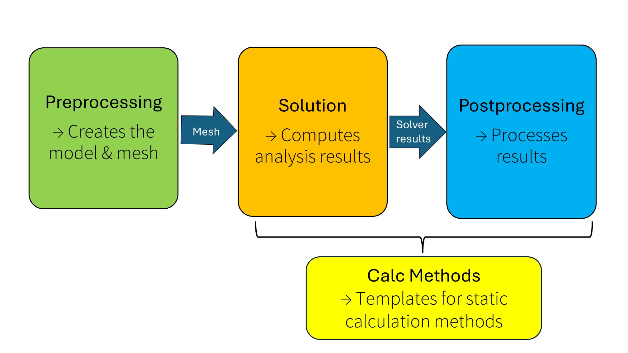
To understand how these steps fit together, let’s walk through a small example.

Example

As a first demonstration, we will model a cantilever beam subjected to a uniform line load. The aim of this example is to show how to:

1. Set up the model

2. Run the structural analysis

3. View and interpret the internal forces diagramm

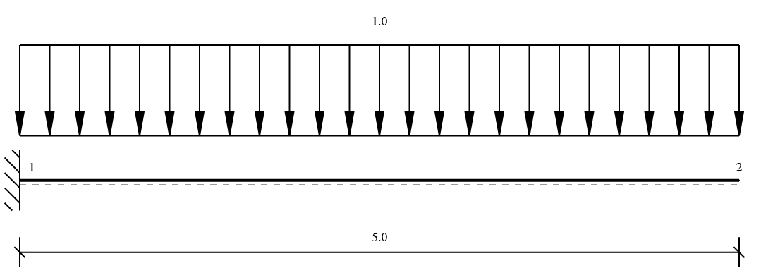
⚠️ Note:

All values are converted into meters (m) and kilonewtons (kN) to keep the units consistent.

Preprocessing

The preprocessing stage is where the structural system is defined. Here you specify the geometry, material, and cross-sections and generate the computational mesh used later in the analysis.

The following diagram shows how the preprocessing classes depend on each other. All classes drawn with a bold outline represent components that you need to create for a complete model.

Step 1: Define material and cross-section

For our cantilever beam, we will use a HEA 240 steel profile together with material S235.

from sstatics.core.preprocessing import CrossSection, Material

# Define material and cross-section
material = Material(210000000, 0.1, 81000000, 0.1)
cross_sec = CrossSection(0.00002769, 0.007684, 0.2, 0.2, 0.1)

Step 2: Define nodes

Every bar element is defined by two nodes. For each node, you need to specify the coordinates and the support conditions.

Support conditions determine how the node can move:

• “free”: the node is not supported in this degree of freedom

• “fixed”: the degree of freedom is fully restrained

• numeric value: defines a spring support with the given stiffness

For our beam example:

• Node 1 is fully fixed: all degrees of freedom (u, w, phi) are set to “fixed”.

• Node 2 remains free: all degrees of freedom use the default setting “free”.

from sstatics.core.preprocessing import Node

# Define nodes
n1 = Node(x=0, z=0, u='fixed', w='fixed', phi='fixed') # fully fixed support
n2 = Node(x=5, z=0) # free end

Step 3: Define the loads

There are several ways to apply loads to a structural system. In the software, loads can act either directly on nodes or along bar elements:

• NodePointLoad: point loads that act directly on a node

• BarLineLoad: line loads acting along the bar (these may be constant or trapezoidal)

• BarPointLoad: a concentrated load applied at any position along a bar

• BarTemp: temperature loads

In our example, the cantilever beam is subjected to a uniform line load in the z-direction. This load is defined using a BarLineLoad object.

from sstatics.core.preprocessing import BarLineLoad

# Define line load
load = BarLineLoad(pi=1, pj=1, direction='z', coord='bar', length='exact')

Step 4: Create the bar and assemble the system

Now that all components are defined, we can create the bar element and build the complete structural system.

A bar is always defined by its start node and end node. In addition, each bar requires a cross-section and a material, since these provide the mechanical properties needed for the later analysis. Loads acting on the bar can be assigned at this stage as well.

When creating the bar, we can simply pass the previously defined nodes, cross-sections, materials, and loads.

Once the bar is created, it is added to the structural system. The order in which bars are added determines their numbering in the system: the first bar added becomes Bar 1, the next becomes Bar 2 and so on.

from sstatics.core.preprocessing import Bar, System

# Define the bar connecting the two nodes
bar_1 = Bar(n1, n2, cross_sec, material, line_loads=load)

# Build the structural system
system = System([bar_1])

from sstatics.core.postprocessing.graphic_objects import ObjectRenderer, SystemGeo

# Show system graphic
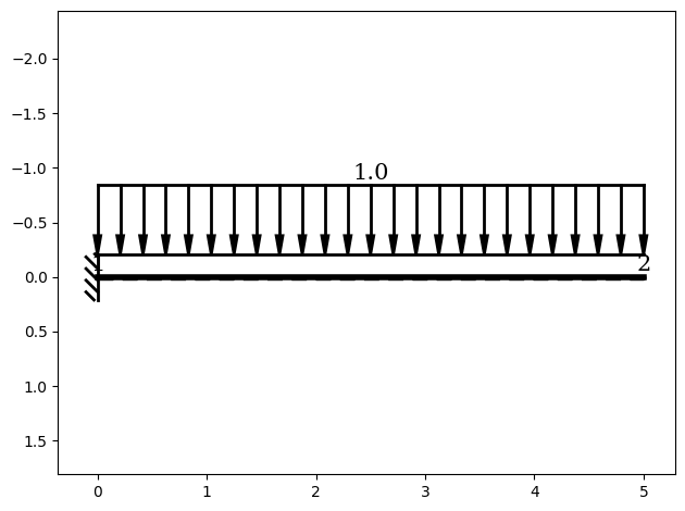
ObjectRenderer(SystemGeo(system), 'mpl').show()

Step 5: Create the mesh

The final step of the modeling process is the creation of the computational mesh. The mesh consists of a list of bar elements that will later be used by the Solver.

The important difference between the modeled bars and the mesh bars is that the mesh takes into account any necessary subdivisions of the bars.

There are two reasons why a bar may be subdivided:

1. Automatic subdivision due to loads

Whenever a BarPointLoad is applied inside a bar (not at the start or end node), the software automatically divides the bar at that load position.

This subdivision is essential because the analysis algorithm evaluates results only at nodes. Without creating a node at the load position, the load could not be correctly included in the calculation.

Example: A single bar with a point load at the midpoint becomes two mesh bars.

This automatic subdivision always takes place and requires no user action.

2. User-defined subdivision

Users may optionally define additional subdivision points along a bar. This can be helpful if results are needed at specific locations. For example, at quarter points or at positions of interest along the structure.

These user-defined divisions are considered during mesh generation and can lead to a mesh that differs from the original list of modeled bars.

Overall, the mesh is a crucial part of the analysis. It ensures that all loads, including point loads inside a bar, are correctly represented and that the solver can evaluate results at all necessary points.

To configure a user_defined division we use the method create_mesh in the System class. In this example we don’t want an additional division. An example demonstrating this subdivision procedure can be found here.

Solution

To compute the internal forces of the system, we pass the System to the Solver. The solver performs all required numerical steps: assembling the stiffness matrix, solving the system of equations and evaluating the structural response.

As output, the solver provides:

• internal forces

• support reactions

• displacements and rotations

• many additional intermediate results

Each calculation step can be inspected in detail, which makes the analysis process transparent and easy to follow.

The illustration below highlights only a small selection of the available solver results. For a full overview, please refer to the API documentation: “API: Solver”

The method internal_forces returns the computed internal forces for each mesh bar.

Important note on sign conventions

When interpreting internal forces, it is essential to understand the sign conventions used during the calculation.

The solver determines the internal forces based on the sign convention defined in the deform method:

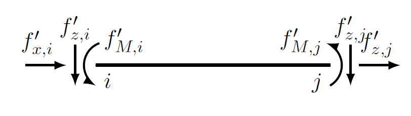
Sign convention used during computation

In hand calculations and in most graphical representations, however, the following sign convention is typically used:

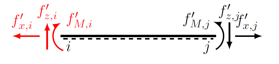
Common sign convention for diagrams and manual calculations

For correct interpretation of the results, it is important to be aware of these two conventions.

All diagrams shown in the Postprocessing stage follow the second sign convention, which corresponds to the standard representation used in structural engineering.

from sstatics.core.solution import Solver

# Perform the structural analysis
solution = Solver(system)

# Extract internal forces of each bar
forces = solution.internal_forces
print("Internal forces of all bars:\n", forces)

Internal forces of all bars:
 [array([[ 0.00000000e+00],
       [-5.00000000e+00],
       [ 1.25000000e+01],
       [ 0.00000000e+00],
       [ 0.00000000e+00],
       [-1.33226763e-15]])]

Analysis of the Results

The following section illustrates how to access and interpret the computed result values in the code.

The internal forces returned by the solver are stored as a list of vectors. Each vector has the dimension 6×1 and contains the internal forces at the start and end of a bar:

1. Normal force at the start node

2. Shear force at the start node

3. Bending moment at the start node

4. Normal force at the end node

5. Shear force at the end node

6. Bending moment at the end node

Accessing the correct vector and entry

Because Python uses 0-based indexing, the bending moment at the start of a bar is located at index [2].

To access a value, two steps are required:

1. Select the correct bar Since the internal forces are stored as a list (one vector per mesh bar), the first bar is accessed using index [0].

2. Select the correct entry Inside the 6×1 vector, you choose the corresponding row. For example, row [2] contains the bending moment at the bar’s start.

If you then want to retrieve the scalar value from this row, select [0] again, because each row is a 1×1 value.

# Each entry is a 6×1 vector: [f'x_i, f'z_i, f'm_i, f'x_j, f'z_j, f'm_j]^T
forces_bar_1 = forces[0]

# 9. Bending moment at node 1 (fixed end)
m_yy = forces_bar_1[2][0]  # index 2 = moment at bar start
print("Bending moment at node 1 [kNm]:", m_yy)

Bending moment at node 1 [kNm]: 12.499999999999996

Post-Processing

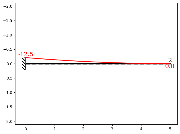
After the solution has been computed, the results can be visualized using the ResultGraphic class.

In this example, we want to display the bending moment diagram of the beam. By setting the parameter kind="moment", the bending moment distribution along the bar is plotted.

The visualization can be generated using either Matplotlib or Plotly. In the figure shown here, the Plotly-based representation is used. Additionally, you can choose which level of subdivision should be displayed:

• the original modeled system (without subdivisions)

• the user-defined subdivisions

• the computational mesh

This flexibility makes it possible to compare the modeled structure with the actual calculation mesh and to inspect the influence of mesh refinement.

Beyond graphical visualization, further postprocessing features are available:

• The class DifferentialEquation allows you to inspect the differential equations of internal force distributions.

A variety of additional examples can be found in the “Examples” section of the documentation.

from sstatics.core.utils import get_differential_equation, plot_results
from sstatics.core.postprocessing.graphic_objects import ObjectRenderer

differential_equation = get_differential_equation(system, solution.bar_deform_total, solution.internal_forces)
system_geo, result_geo = plot_results(system, differential_equation, 'moment', decimals=1)
ObjectRenderer([system_geo, result_geo], 'mpl').show()

Calculation Methods

To simplify the workflow for users, templates for static calculation methods have been provided. These templates allow you to:

• automatically create the computational mesh

• perform the analysis

• generate plots directly from the calculation class

The calculation classes serve as a bridge between the Solution and Post-Processing stages, enabling a more efficient workflow and faster setup of analysis tasks.

Several example implementations of these calculation methods can be found in the “Examples” section of the documentation.

Next Steps

You have now completed your first example and seen how to:

• define a structural system, materials, and loads,

• create the computational mesh,

• run the analysis using the Solver,

• visualize and interpret the results.

From here, you can explore more advanced topics, such as:

• applying different types of loads,

• analyzing more complex structures,

• using the calculation method templates for automated workflows.

For additional guidance and more examples, please visit the “Examples” section of the documentation.