Principle of Virtual Forces: Relative Rotation

Computing the relative rotation of two bars at a shared node using the Principle of Virtual Forces (PVF)

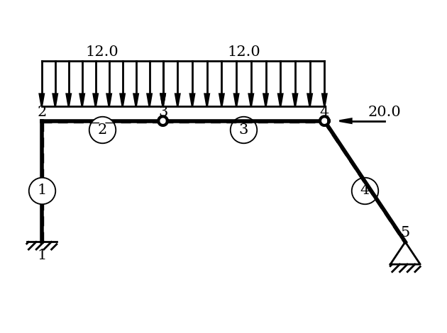
In this example, the relative rotation (phi) of bars 1 and 2 at the common node_3 is computed. Individual deformation contributions can be specified for each bar using the deformations attribute.

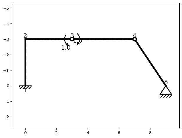
The PVF method introduces a virtual moment couple on the two bars at the connecting node. Evaluating the work equation yields the desired relative rotation.

You can find the example as an executable Python file here.

Define the Structural System

In this section, the static system is modeled. For a detailed step-by-step workflow, refer to the “Getting Started” example.

# 1. Import modules
from sstatics.core.preprocessing import (
    Bar, BarLineLoad, CrossSection, Material, Node, NodePointLoad, System
)
from sstatics.core.calc_methods import PVF
from sstatics.core.postprocessing.graphic_objects import ObjectRenderer, SystemGeo
import numpy as np

# 2. Define material
s253 = Material(210000000, 0.1, 81000000, 0.1)

# 3. Define cross-sections
ipe_360 = CrossSection(16270 * 1e-8, 72.7 * 1e-4, 0.360, 0.170, 5/6)
ipe_220 = CrossSection(2772 * 1e-8, 33.4 * 1e-4, 0.240, 0.120, 5/6)

# 4. Define nodes
n1 = Node(0, 0, u='fixed', w='fixed', phi='fixed', rotation=np.pi/2)
n2 = Node(0, -3)
n3 = Node(3, -3)
n4 = Node(7, -3, loads=[NodePointLoad(x=-20)])
n5 = Node(9, 0, u='fixed', w='fixed')

# 5. Define loads and deformation components
line_load = BarLineLoad(pi=12, pj=12)
def_comp = 'moment'

# 6. Define bars
b1 = Bar(n1, n2, ipe_360, s253, deformations=def_comp)
b2 = Bar(n2, n3, ipe_360, s253, line_loads=line_load, deformations=def_comp)
b3 = Bar(n3, n4, ipe_220, s253, hinge_phi_i=True, hinge_phi_j=True,
         line_loads=line_load, deformations=def_comp)

b4 = Bar(n4, n5, ipe_220, s253, deformations=def_comp)

# 7. Assemble system
system = System(bars=[b1, b2, b3, b4])

# Visualize system
ObjectRenderer(SystemGeo(system, show_bar_text=True), 'mpl').show(show_axis=False)

Perform the Principle of Virtual Forces

Next, we pass the modeled system to the PVF class to perform the principle of virtual forces.

# 6. Compute displacement using Principle of Virtual Forces (PVK)
pvf = PVF(system)

Create a Virtual Load System

A virtual load must now be applied at the location where the deformation is to be evaluated. There are three available options for defining the virtual load:

1. ``add_virtual_node_load`` – apply a nodal load

2. ``add_virtual_bar_load`` – apply a bar point load

3. ``add_virtual_moment_couple`` – apply a virtual moment couple

⚠️ Note: Only one virtual load may be applied in the virtual system.

In this example, the goal is to compute the relative rotation at node 3. Therefore, a virtual moment couple has to be applied on bar 2 and bar 3 with their shared node 3. With this, the virtual system is fully defined.

# Apply a virtual moment couple on bars 2 and 3 at node 3
pvf.add_virtual_moment_couple(
    bar_positive_m=b2,
    bar_negative_m=b3,
    connecting_node=n3
)

# Show virtual system
ObjectRenderer(SystemGeo(pvf.virtual_system), 'mpl').show()

Plot of the Bending Moment Distribution

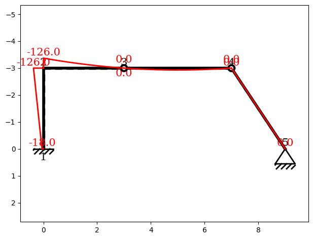
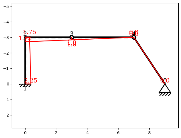
It is also possible to visualize the results of the system under real loads and virtual loads graphically. This is done in a similar way to the FirstOrder class. The key difference is which ``mode`` is selected for the plot.

Plot of the System under Real Loads

The bending moment distribution for the real loading case can be generated by setting the mode to "real":

# Plot moment distribution
pvf.plot('real', kind='moment')

Plot of the System under Virtual Loads

# Plot moment distribution
pvf.plot('virt', kind='moment')

Retrieve the Desired Deformation

The requested deformation can now be obtained using the deformation() function. Depending on the material properties, cross-section parameters and the nodal coordinates provided, the deformation is returned in the corresponding unit.

delta_phi = pvf.deformation()
print("Relative rotation at node 3 (PVK) [rad]:", delta_phi)

Relative rotation at node 3 (PVK) [rad]: -0.013962417893778667

Evaluation of Work Contribution

It is possible to analyze how individual contributions affect the work equation. The provided functions give an inside the contribution for all bars or all nodes, showing how the total deformation is influenced by each type of load or internal force.

This gives a deeper understanding of the calculation, highlighting which contributions dominate the deformation.

Work Contribution of Bars

The work_matrix function calculates the contributions of the bars. Each column represents a specific type of contribution:

1. Bending moment

2. Normal force

3. Shear force

4. Constant temperature (\(T_s\))

5. Non-uniform temperature change (\(\Delta_T\))

Each row represents a bar of the mesh.

This allows you to see how the total bar deformations result from each type of contribution.

# Work matrix for bars
# for better visualization change print options
import numpy as np
np.set_printoptions(
    suppress=True,    # suppress scientific notation for small numbers
)

work_matrix_bars = pvf.work_matrix(kind='bars')
print("Work matrix (bars):\n", work_matrix_bars)

Work matrix (bars):
 [[-0.01224866  0.          0.          0.          0.        ]
 [-0.00721091  0.          0.          0.          0.        ]
 [ 0.00549715  0.          0.          0.          0.        ]
 [-0.          0.          0.          0.          0.        ]]

Work Contribution of Nodes

Next, we examine the work matrix for the nodes.

The columns represent the following contributions:

1. Contribution from elastic translational supports

2. Contribution from elastic rotational supports

3. Contribution from the nodal displacements (NodeDisplacement)

4. Contribution from the nodal rotations (NodeDisplacement)

Each row represent a node.

# Work matrix for nodes
work_matrix_nodes = pvf.work_matrix(kind='nodes')
print("Work matrix (nodes):\n", work_matrix_nodes)

Work matrix (nodes):
 [[0. 0. 0. 0.]
 [0. 0. 0. 0.]
 [0. 0. 0. 0.]
 [0. 0. 0. 0.]
 [0. 0. 0. 0.]]

Work Contribution of a Specific Bar or Node

It is also possible to examine the contributions for individual bars or nodes. For this purpose, the modeled bar or node is passed to the function work_of.

In this example, we analyze the work contributions of bar 1.

# If we want to query the specific contribution of a single model object
# to the work equation, we can use the `work_of(...)` method.
work_b4 = pvf.work_of(obj=b1)
print("Work contribution of bar 1:\n", work_b4)

Work contribution of bar 1:
 [-0.01224866  0.          0.          0.          0.        ]