Reduction Theorem: Large statically indeterminate frame

Computing a deformation in a large statically indeterminate frame using the Reduction Theorem

In this example, a large statically indeterminate frame is analyzed. The system has multiple redundants, and the Reduction Theorem is used to remove them by releasing specific degrees of freedom (hinges or node releases), forming a statically determinate system.

After removing the redundant constraints, the deformation at a specific location is computed directly using the Reduction Theorem. A hand-calculated reference value using integration formulas is also provided to validate the numerical result.

This example demonstrates the application of the Reduction Theorem in complex frames with high degrees of static indeterminacy, without introducing additional virtual loads.

You can find the example as an executable Python file here.

Define the Structural System

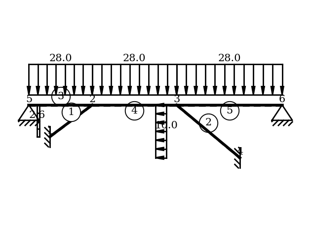
In this section, the static system is modeled. For a detailed step-by-step workflow, refer to the “Getting Started” example.

# 1. Import required modules
from sstatics.core.calc_methods import ReductionTheorem
from sstatics.core.preprocessing import (
    Node, Bar, Material, CrossSection, System, BarLineLoad, Polygon
)
from sstatics.core.postprocessing.graphic_objects import ObjectRenderer, SystemGeo
import numpy as np

# 2. Define material
material = Material(3300e4, 1, 1, 1)

# 3. Define cross-sections using polygon geometry
rect_1 = Polygon(points=[(0, 0), (0.35, 0), (0.35, 0.35), (0, 0.35), (0, 0)])
rect_2 = Polygon(points=[(0, 0), (0.35, 0), (0.35, 0.6), (0, 0.6), (0, 0)])

cs_1 = CrossSection(geometry=[rect_1])
cs_2 = CrossSection(geometry=[rect_2])

# 4. Define nodes
node_a = Node(0, 3, u='fixed', w='fixed', phi='fixed')
node_b = Node(18, 5, u='fixed', w='fixed', phi='fixed')
node_c = Node(-2, 0, u='fixed', w='fixed')
node_d = Node(4, 0)
node_e = Node(12, 0)
node_f = Node(22, 0, u='fixed', w='fixed')

# 5. Define bar loads
line_load_1 = BarLineLoad(pi=28, pj=28, direction='z')
line_load_2 = BarLineLoad(pi=2.6, pj=2.6, direction='x', coord='system',
                          length='proj')
line_load_3 = BarLineLoad(pi=-10, pj=-10, direction='x', coord='system',
                          length='proj')

# 6. Define bars
bar_1 = Bar(node_a, node_d, cs_1, material, line_loads=line_load_2,
            deformations="moment")
bar_2 = Bar(node_e, node_b, cs_1, material, line_loads=line_load_3,
            deformations="moment")
bar_3 = Bar(node_c, node_d, cs_2, material, line_loads=line_load_1,
            deformations="moment")
bar_4 = Bar(node_d, node_e, cs_2, material, line_loads=line_load_1,
            deformations="moment")
bar_5 = Bar(node_e, node_f, cs_2, material, line_loads=line_load_1,
            deformations="moment")

# 7. Define system
system = System([bar_1, bar_2, bar_3, bar_4, bar_5])

# Visualize system
ObjectRenderer(SystemGeo(system, show_bar_text=True), 'mpl').show(show_axis=False)

Perform the Reduction Theorem

Next, we pass the modeled system to the ReductionTheorem class.

# 8. Create ReductionTheorem instance
red = ReductionTheorem(system)

Determine the Degree of Static Indeterminacy

Before creating a released system, it is necessary to determine the degree of static indeterminacy. This value can be obtained using the function degree_of_static_indeterminacy.

For our modeled system, the degree of static indeterminacy is:

print("Degree of static indeterminacy:",
      red.degree_of_static_indeterminacy)

Degree of static indeterminacy: 7

Create Released System

We now know that our modeled system is statically indeterminate of degree 7. The released system represents the corresponding statically determinate system of the original model.

To obtain such a system, certain restraints must be released. However, it is essential that the structure remains stable after doing so.

There are three available methods:

• ``modify_node()`` Modifies a support condition. The modeled node is passed to the function, and the specific degree of freedom to be released is defined.

• ``modify_bar()`` Modifies a bar by introducing a hinge. The modeled bar is passed to the function, and a hinge is added to release the corresponding internal restraint.

• ``delete_bar()`` Removes a bar from the structure. However, the software does not internally check the deformation contributions to verify whether removing a bar is structurally safe.

# 9. Remove redundant degrees of freedom to form a statically determinate
# system
red.modify_node(node_a, 'phi')
red.modify_bar(bar_3, 'hinge_phi_j')
red.modify_bar(bar_4, 'hinge_phi_j')
red.modify_bar(bar_1, 'hinge_phi_j')
red.modify_bar(bar_2, 'hinge_phi_i')
red.modify_node(node_b, 'phi')
red.modify_node(node_f, 'u')

Check the Degree of Static Indeterminacy Again

Now we check the degree of static indeterminacy once more to verify that it is now equal to 0. A value of 0 indicates that the system is statically determinate, meaning the released system has been successfully created.

print("Degree of static indeterminacy (after):",
      red.degree_of_static_indeterminacy)

Degree of static indeterminacy (after): 0

The released system is now statically determinate.

Plot the Released System

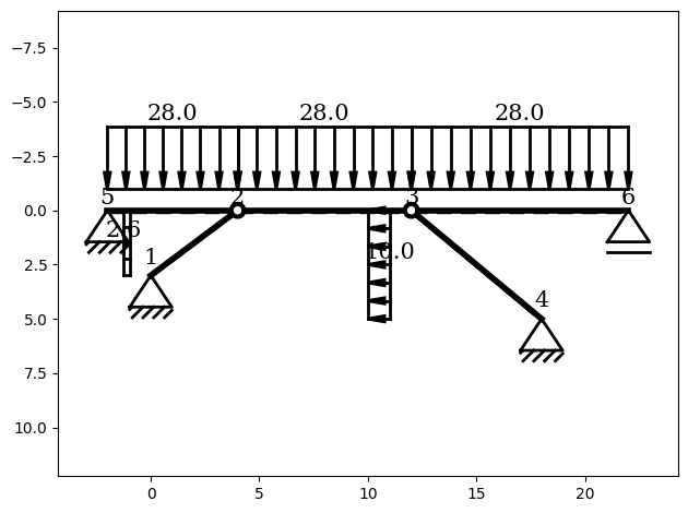
It is possible to visualize the released system using plot_released_system(). This allows you to inspect the modified structure and verify which connections or supports were released.

# Show the released system
red.plot_released_system()

Create a Virtual Load System

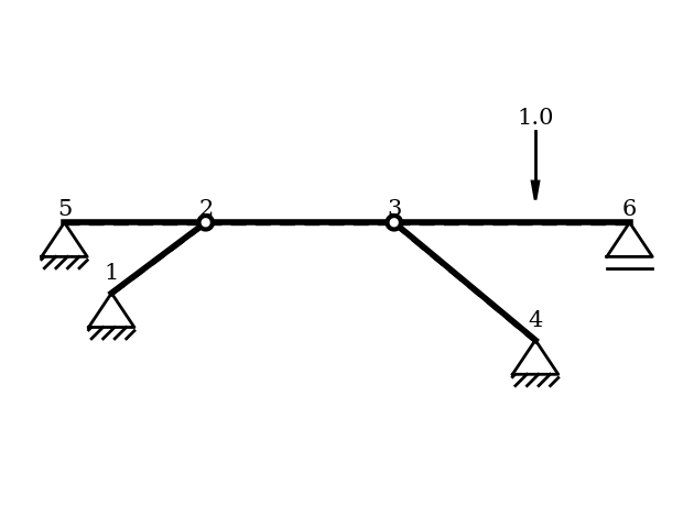
Once the released system has been fully created, we can generate the corresponding virtual load system based on it.

A virtual load must be applied at the exact location where the deformation is to be evaluated. There are three options for defining such a virtual load:

1. ``add_virtual_node_load`` – apply a virtual nodal load

2. ``add_virtual_bar_load`` – apply a virtual load directly to a bar

3. ``add_virtual_moment_couple`` – apply a virtual moment couple

⚠️ Note: Only one virtual load may be applied in the virtual system.

In this example, the goal is to compute the vertical deformation of bar 5. Therefore, a virtual bar load in the z-direction is applied at the relative position 0.6 along the bar. With this step, the virtual system is fully defined.

# 8. Apply a virtual unit vertical load at Bar 5
red.add_virtual_bar_load(bar_5, 'fz', position=0.6)

# Show virtual system
ObjectRenderer(SystemGeo(red.virtual_system), 'mpl').show(show_axis=False)

Retrieve the Desired Deformation

The requested deformation can now be obtained using the deformation() function. Depending on the material properties, cross-section parameters and the nodal coordinates provided, the deformation is returned in the corresponding unit.

# 10. Compute deformation directly at bar_5
delta_dv_sstatics = red.deformation()
print("Deformation (ReductionTheorem):", delta_dv_sstatics)

Deformation (ReductionTheorem): 0.00894319499313046

Verify the Results

In the next step, we verify the computed deformation to ensure its correctness. To do this, the hand-calculation is replicated using integration tables. For the manual evaluation, the moment diagrams of both systems are needed:

• the original system with real loads, and

• the released system with the applied virtual load.

To obtain these moment distributions, both systems are plotted with their corresponding bending moment diagrams. These plots allow a direct comparison between the numerical results and the hand-calculated integration approach.

# 10. Hand calculation using classical integration tables
red.plot('real', kind='moment')
red.plot('virt', kind='moment')

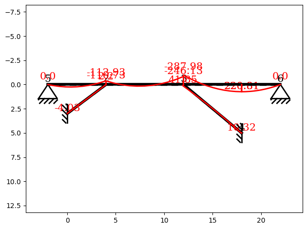
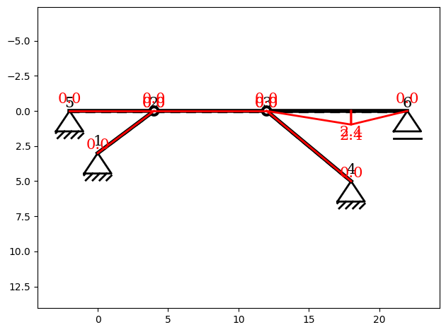
To compute the deformation, the moment areas are now superimposed using the formulas from the integration tables.

delta_dv_seminar = (1/4 * 2.4 * (-288) * 10 / 207900 +
                    5/12 * 2.4 * 350 * 10 / 207900)

print("Deformation (Hand calculation):", delta_dv_seminar)

Deformation (Hand calculation): 0.008523328523328525

Comparison of the Two Methods

The deformations obtained from both methods can now be compared.

# 12. Verify equality
print("Results match:",
      np.allclose(delta_dv_sstatics, delta_dv_seminar, atol=1e-3))

Results match: True

This demonstrates that the results from both methods match, confirming the validity of the calculations.