Principle of Virtual Forces: Basic Example

Computing the displacement w at a node using the Principle of Virtual Forces (PVF)

In this example, the vertical displacement w at node_2 of a cantilever beam is computed using two independent methods:

1. The displacement method (FirstOrder)

2. The Principle of Virtual Forces (PVF)

The principle of virtual forces provides a powerful and elegant way to determine displacements by introducing a virtual load in the direction and at the location of the desired displacement. Evaluating the work equation yields the desired deformation.

To validate the PVF result, the same displacement w at node_2 is computed using the FirstOrder solver. The results of both methods are compared and verified to be equal within numerical tolerance.

You can find the example as an executable Python file here.

Define the Structural System

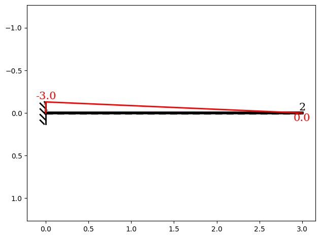
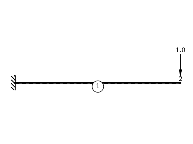
In this section, the static system is modeled. The structural system used in this example is introduced in “First-Order: Bending Moment”. For a detailed step-by-step workflow, refer to the “Getting Started” example.

# 1. Import required modules
from sstatics.core.preprocessing import (
    Bar, CrossSection, Material, Node, NodePointLoad, System
)
from sstatics.core.preprocessing.geometry import Polygon
from sstatics.core.calc_methods import FirstOrder, PVF
from sstatics.core.postprocessing.graphic_objects import ObjectRenderer, SystemGeo
import numpy as np

# 2. Define cross-section using polygon geometry
cs_1 = CrossSection(
    geometry=[Polygon([(0, 0), (0.1, 0), (0.1, 0.2), (0, 0.2), (0, 0)])]
)

# 3. Define material (E = 11,000,000 kN/m²)
mat_1 = Material(11000000, 0.1, 0.1, 0.1)

# 4. Define nodes
n1 = Node(0, 0, u='fixed', w='fixed', phi='fixed')  # Fixed support
n2 = Node(3, 0, loads=NodePointLoad(z=1))  # Real vertical load at free end

# 5. Define bar and system
bar = Bar(n1, n2, cs_1, mat_1)
system = System([bar])

# Visualize system
ObjectRenderer(SystemGeo(system, show_bar_text=True), 'mpl').show(show_axis=False)

Perform the Principle of Virtual Forces

Next, we pass the modeled system to the PVF class to perform the principle of virtual forces.

# 6. Compute displacement using Principle of Virtual Forces (PVK)
pvf = PVF(system)

Create a Virtual Load System

A virtual load must now be applied at the location where the deformation is to be evaluated. There are three available options for defining the virtual load:

1. ``add_virtual_node_load`` – apply a nodal load

2. ``add_virtual_bar_load`` – apply a bar point load

3. ``add_virtual_moment_couple`` – apply a virtual moment couple

⚠️ Note: Only one virtual load may be applied in the virtual system.

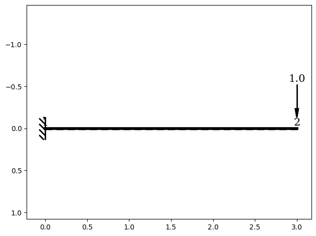
In this example, the goal is to compute the vertical deformation at the end of the bar. Therefore, a virtual bar load in the z-direction is applied. With this, the virtual system is fully defined.

# For displacement w at node_2:
# → Apply a virtual vertical force fz at the bar end (position=1)
pvf.add_virtual_bar_load(obj=bar, force='fz', position=1)

# Show virtual system
ObjectRenderer(SystemGeo(pvf.virtual_system), 'mpl').show()

Retrieve the Desired Deformation

The requested deformation can now be obtained using the deformation() function. Depending on the material properties, cross-section parameters and the nodal coordinates provided, the deformation is returned in the corresponding unit.

w_node_2_pvf = pvf.deformation()
print("w at node 2 (PVK) [m]:", w_node_2_pvf)

w at node 2 (PVK) [m]: 0.012272727272727262

Calculate Deformation with First-Order Analysis

To validate the deformation obtained using the principle of virtual forces, we compute the same value using the FirstOrder solver. The bar deformations can be retrieved using the function bar_deform_total.

Since we are interested in the vertical deformation at the end of the bar, index 4 is used. For a detailed explanation of bar deformation indexing, refer to the example: “First-Order: Bar Deflection”.

# 7. Compute displacement using FirstOrder method
solution = FirstOrder(system)

# Extract deformation vector of the single bar (index 0)
bar_deform = solution.bar_deform_total[0]

# Vertical displacement w at node_2 is located at index 4
w_node_2 = bar_deform[4][0]
print("w at node 2 (FirstOrder) [m]:", w_node_2)

w at node 2 (FirstOrder) [m]: 0.012272727272727267

Validate Results of Both Methods

The results from both approaches can now be compared. Both methods should yield the same deformation value. Thus, both methods provide matching deformation results, validating the implementation and the structural model.

# 8. Verify equality of both methods
print("Results match:", np.allclose(w_node_2, w_node_2_pvf))

Results match: True

Plot of the Bending Moment Distribution

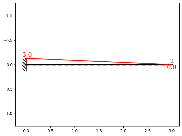
It is also possible to visualize the results of the system under real loads and virtual loads graphically. This is done in a similar way to the FirstOrder class. The key difference is which ``mode`` is selected for the plot.

Plot of the System under Real Loads

The bending moment distribution for the real loading case can be generated by setting the mode to "real":

# 9. Plot moment distribution
pvf.plot('real', kind='moment')

Plot of the System under Virtual Loads

# 9. Plot moment distribution
pvf.plot('virt', kind='moment')