Poleplan: Advanced

The following example demonstrates how a poleplan object can be created from a system object.

Finally, the poleplan is visualized.

You can find the example as an executable Python file here.

Import Modules

We start by importing the required classes for defining and visualizing the poleplan.

from sstatics.core.preprocessing import (Node, Bar, Material, CrossSection, System)
from sstatics.core.solution import Poleplan
from sstatics.core.postprocessing.graphic_objects import ObjectRenderer, SystemGeo

Define System

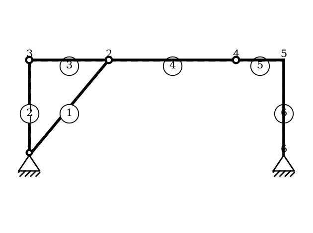
Here, we only show the system modeling in a concise form, without additional explanations.

# define cross-section
c_1 = CrossSection(mom_of_int=2769, area=76.84, height=20, width=10, shear_cor=0.1)

# define material
m_1 = Material(young_mod=21000, poisson=0.1, shear_mod=8100, therm_exp_coeff=0.1)

# define Node
node_1 = Node(0, 0, u='fixed', w='fixed')
node_2 = Node(0, -3)
node_3 = Node(2.5, -3)
node_4 = Node(6.5, -3)
node_5 = Node(8, -3)
node_6 = Node(8, 0, u='fixed', w='fixed')

# define Bar
bar_1 = Bar(node_1, node_3, c_1, m_1, hinge_phi_j=True)
bar_2 = Bar(node_1, node_2, c_1, m_1, hinge_phi_i=True, hinge_phi_j=True)
bar_3 = Bar(node_2, node_3, c_1, m_1, hinge_phi_j=True)
bar_4 = Bar(node_3, node_4, c_1, m_1, hinge_phi_j=True)
bar_5 = Bar(node_4, node_5, c_1, m_1)
bar_6 = Bar(node_5, node_6, c_1, m_1)

bars = [bar_1, bar_2, bar_3, bar_4, bar_5, bar_6]

# define System
system = System(bars)

# Visualize system
ObjectRenderer(SystemGeo(system, show_bar_text=True), 'mpl').show(show_axis=False)

Define Poleplan

The poleplan can be accessed directly as an attribute of the System class:

poleplan = Poleplan(system=system)

Visualize Poleplan

We can visualize the Poleplan using the plot() method of th class.

This allows us to see the kinematic configuration of the system.

poleplan.plot()

Result:

The diagram shows the poleplan and the displacement figure (in red).

The kinematic chain consists of three chains:

• Chain 1 (shown in purple) has its absolute pole at Node 1 (0, 0).

• Chain 2 (shown in green) has its absolute pole at (5, -6).

• Chain 3 (shown in yellow) has its absolute pole at node 6 (8, 0).

• The relative pole (1|2) is located at Node 3 (2.5, -3).

• The relative pole (2|3) is located at Node 4 (6.5, -3).

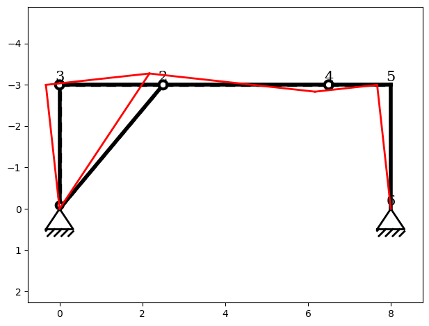
In this step we visualize the rigid-body displacement of the system. By default, the rotation of the first chain is set to a value of 1, which provides a normalized reference deformation for the entire mechanism. This default setting helps to illustrate how the remaining chains react when the system undergoes an imposed unit rotation.

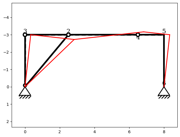
To study the influence of a different rotation on a specific chain, we can manually assign an angle to any chain within the structure. The following command shows how to adjust the rotation of the chain with index 1:

poleplan.set_angle(chain_idx=1, angle=0.2)

Here:

• chain_idx=1 selects the chain to be modified,

• angle=0.2 sets its rotation to a value of`0.2 (in radians, unless defined otherwise).

By changing this angle, we can investigate how the system’s geometry and kinematics respond to a modified rigid-body rotation. This is particularly useful for understanding displacement figures, visualizing the kinematic behavior of the structure, and analyzing influence lines derived from the polar diagram.

poleplan.plot()