
Second Order: Matrix Approach#
Comparison of the bending moment at the fixed end for different matrix-based second-order methods and in comparison to first-order analysis
In this example, we demonstrate the differences between First-Order and Second-Order structural analysis for a cantilever column. Additionally, the example compares the results of the matrix-based geometric-nonlinear approaches, showing how different computational variants influence the bending moment at the fixed support.
The example illustrates:
Modeling a cantilever column with cross-section and material properties
Applying point and distributed loads
Running first-order and second-order computations
Understanding how the Solver incorporates geometric nonlinearity
Comparing the bending moment at the base for different calculation approaches
System Description#
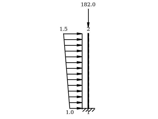
We consider a 4 m high cantilever column with an HEA 240 profile. The column is subjected to a concentrated load at its free end and a trapezoidal distributed load along the entire height.
Length: 4 m - Cross-section: HEA 240
\(I\) = 2769 cm\(^4\)
\(A\) = 76.84 cm\(^2\) - \(\kappa\) = 0.6275377
Material: S 235 (Steel) - \(E\) = 21 000 \(\frac{\text{kN}}{\text{cm}^2}\)
\(G\) = 8 100 \(\frac{\text{kN}}{\text{cm}^2}\)
Loads:
Point load at the top: \(P\) = 182 kN
Trapezoidal distributes load over the entire length
You can find the example as an executable Python file here.
Define the Structural System#
In this section, the static system is modeled. For a detailed step-by-step workflow, refer to the “Getting Started” example.
[1]:
from sstatics.core.preprocessing import (Bar, BarLineLoad, CrossSection,
                                         Material, Node, NodePointLoad, System)
from sstatics.core.calc_methods import SecondOrder, FirstOrder
from sstatics.core.postprocessing.graphic_objects import ObjectRenderer, SystemGeo
import numpy as np

# 1. Define cross-section and material -> steel and HEA 240 profile
c_1 = CrossSection(0.00002769, 0.007684, 0.2, 0.2, 0.6275377)
m_1 = Material(210000000, 0.1, 81000000, 0.1)

# 2. Define nodes (cantilever system)
node_1 = Node(x=0, z=0, u='fixed', w='fixed', phi='fixed', rotation=np.pi/2)
node_2 = Node(x=0, z=-4, loads=NodePointLoad(x=0, z=182, phi=0, rotation=0))

# 3. Define bar
bar_1 = Bar(node_1, node_2, c_1, m_1, line_loads=BarLineLoad(
    pi=1, pj=1.5, direction='z', coord='bar', length='exact'))

# 4. Define system
system = System([bar_1])

# Show system graphic
ObjectRenderer(SystemGeo(system), 'mpl').show(show_axis=False)
First-Order Analysis#
In the first step, the system is solved according to First-Order Theory (linear analysis). This step provides for example displacements and internal forces without considering geometric nonlinearities. To see a detailled list of all the possible results of the First-Order Analysis go to API References of FirstOrder. The displacements and internal forces are obtained for small deformations. These serve as the basis for the Second-Order analysis.
[2]:
# Get Solution Instance
solution_first_order = FirstOrder(system)
Transition to Second-Order Theory#
The Second-Order Theory accounts for geometric nonlinear effects, such as P–Δ effects. The computational procedure is as follows:
Initial Solution:
The system is first solved using the standard
Solverto obtain the internal forces and deformations of the bar, which are important to calculate the average axial force.
Average Axial Force:
The average longitudinal (axial) force in each bar is computed by the use of the method
averaged_longitudinal_force.This force is used to modify the stiffness matrices and load vectors.
Bar Conversion:
Using the method
_convert_bars, each bar of classBaris converted into aBarSecondOrder.These new elements contain the nonlinear geometric terms.
System Assembly
The converted
BarSecondOrderelements are assembled into a new system.The topology remains the same, but now the system includes geometric nonlinear behavior.
System Solution
The new system can be solved again using the
SolverClass
To simplify the workflow, dedicated methods are provided to create Solver objects according to the selected approach. To perform the calculation using the matrix-based approach, call matrix_approach() and select a calculation variant. The available variants are:
analytic: Analytical matrix formulationtaylor: Taylor series approximationp_delta: Simplified P–Δ approach
[3]:
# 6. Create a SecondOrder object
sec_order = SecondOrder(system)

# 7. Set matrix approach and a chosen variant and get solver object
# analytic
sec_order.matrix_approach('analytic')
solution_analytic = sec_order.solver_matrix_approach
After calling matrix_approach, you can access the Solver via solver_matrix_approach or the modified system via system_matrix_approach. These methods are useful for inspecting local stiffness matrices and to get internal forces and deformations according to Second-Order Theory. The system or solver instance cannot be accessed before calling matrix_approach. If a different calculation variant is selected, the results from the previous variant are discarded, and the new approach
is applied for both system_matrix_approach and solver_matrix_approach.
Transformation of Internal Forces#
The internal forces returned by the solver (internal_forces) are expressed as equivalent longitudinal and transverse components. To obtain the actual normal and shear forces, these values must be transformed back into the local bar coordinate system using the method _transform_internal_forces().
If you are already using the solver_matrix_approach function, this transformation is performed automatically.
Comparison of First- and Second-Order Results#
For the calculation variants “taylor” and “p_delta”, the corresponding solutions must also be obtained using solver_matrix_approach in order to create a consistent comparison with the first-order analysis.
Comparing the Bending Moment at the Start of the Bar#
To extract the bending moment at the start of the bar, the values from internal_forces must be evaluated. A detailed explanation of the indexing required to retrieve bending moments can be found in the example: “First-Order: Bending Moment”.
[4]:
# taylor
sec_order.matrix_approach('taylor')
solution_taylor = sec_order.solver_matrix_approach

# p-delta
sec_order.matrix_approach('p_delta')
solution_p_delta = sec_order.solver_matrix_approach

# 8. Get moment at the beginning of the bar
moment_analytic = solution_analytic.internal_forces[0][2][0]
moment_taylor = solution_taylor.internal_forces[0][2][0]
moment_p_delta = solution_p_delta.internal_forces[0][2][0]
moment_first = solution_first_order.internal_forces[0][2][0]

print("=== Second Order Example - comparing results===")
print(f'Mi - first order: {moment_first} [kNm]')
print(f'Mi - second order analytic: {moment_analytic} [kNm]')
print(f'Mi - second order taylor: {moment_taylor} [kNm]')
print(f'Mi - second order p delta: {moment_p_delta} [kNm]')
=== Second Order Example - comparing results===
Mi - first order: 10.666666666666709 [kNm]
Mi - second order analytic: 12.369294641439046 [kNm]
Mi - second order taylor: 12.373174522851505 [kNm]
Mi - second order p delta: 12.30973930064128 [kNm]
⚠️ Note:It should be noted that the sign convention is determined according to the deformation method.
Conclusion#
The Second-Order Theory enables the consideration of geometric nonlinearities and provides more realistic results, especially for slender structural members. The use of BarSecondOrder and the corresponding solvers allows flexible and accurate structural analysis.