Stress: Plotting Normal Stress

In this example, we demonstrate how to plot the normal stress distribution along a cross-section.

This combines the previous calculations of normal stress with a graphical visualization.

You can find the example as an executable Python file here.

Create Stress-Object

We create an instance of CrossSectionStress.

from sstatics.core.preprocessing import CrossSection
from sstatics.core.preprocessing.geometry.objects import Polygon
from sstatics.core.postprocessing import CrossSectionStress

# 1. Create a simple rectangular cross-section (width 10, height 40)
rect = Polygon(points=[(0, 0), (10, 0), (10, 40), (0, 40), (0, 0)])
cs = CrossSection(geometry=[rect])

# 2. Create stress calculator
stress = CrossSectionStress(cs)

# 3. Example loads
N = 1000

Discretize the Stress for Plotting

Before plotting, we must call the *_disc() method:

disc_values = stress.normal_stress_disc(n=N)
print(disc_values)

[[np.float64(0.0), np.float64(40.0)], [np.float64(2.5), np.float64(2.5)]]

This method:

• Computes stress values at discrete points along the section height,

• Stores the results internally, ready for plotting. The structure of disc_values is:

[
  [z-values],         # positions along the height
  [stress-values]     # corresponding sigma at each position
]

Plot the Normal Stress Distribution

Finally, we plot the stored stress distribution using:

stress.plot(kind='normal')

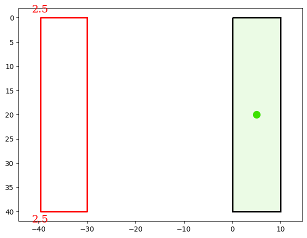
This produces a graphical representation of the normal stress \(\sigma\) along the height of the cross-section, allowing easy visualization of how the axial load affects different parts of the section.