First-Order: Bending Moment

Determining the bending moment at the fixed support of a cantilever beam

In this example, we analyze a simple cantilever beam using first-order structural analysis. A point load is applied at the free end, and the resulting internal forces and support reactions are computed.

This example demonstrates:

• Defining a cross-section from polygon geometry

• Modeling a beam with a fixed support and a free-end load

• Extracting internal forces from the calculation results

• Reading the bending moment at the fixed support

• Accessing support reactions directly

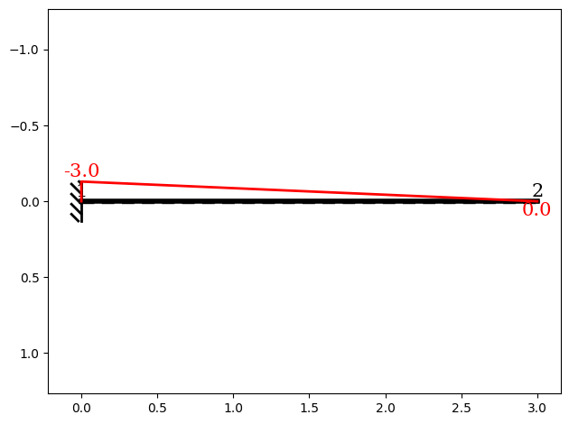
• Plotting the bending moment distribution

This serves as a minimal introduction to the basic workflow of sStatics. You can find the example as an executable Python file here.

System Description

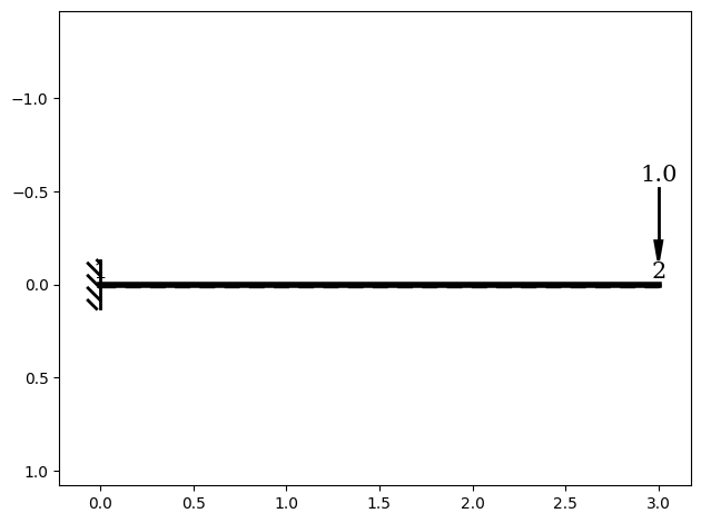
• Beam length: 3 m

• Material: Timber C24, (E = 11000000 \(\frac{kN}{m^2}\))

• Cross-section: width / height = 10 cm / 20 cm

• Support: fixed at the left end (Node 1)

• Load: 1 kN vertical point load at the free end (Node 2)

⚠️ Note: All values are converted into meters (m) and kilonewtons (kN) for consistent units.

Define the Structural System

In this section, the static system is modeled. For a detailed step-by-step workflow, refer to the “Getting Started” example.

# 1. Import required modules
from sstatics.core.preprocessing import (
    Bar, CrossSection, Polygon, Material, Node, NodePointLoad, System
)
from sstatics.core.calc_methods import FirstOrder
from sstatics.core.postprocessing.graphic_objects import ObjectRenderer, SystemGeo

# 2. Define the cross-section using polygon geometry
cross_sec = CrossSection(
    geometry=[Polygon([(0, 0), (0.1, 0), (0.1, 0.2), (0, 0.2), (0, 0)])]
)

# 3. Define material (E = 11,000,000 kN/m²)
material = Material(11000000, 0.1, 0.1, 0.1)

# 4. Define nodes
n1 = Node(0, 0, u='fixed', w='fixed', phi='fixed')  # fully fixed support
n2 = Node(3, 0, loads=NodePointLoad(z=1))  # free end with load

# 5. Define the bar connecting the two nodes
bar_1 = Bar(n1, n2, cross_sec, material)

# 6. Build the structural system
system = System([bar_1])

# Show system graphic
ObjectRenderer(SystemGeo(system), 'mpl').show()

Perform the Structural Analysis

Next, we assemble the bar into a structural system and perform a first-order analysis.

The FirstOrder class differs from the standard Solver in that it accepts the structural system directly, rather than a pre-defined mesh. The computational mesh is generated automatically during the analysis, so you can focus on defining the model and loads.

This approach simplifies the workflow and allows you to quickly compute internal forces, support reactions and other results without manually creating the mesh.

# 7. Perform first-order structural analysis
solution = FirstOrder(system)

Get the Internal Forces

The internal forces are accessed using the function internal_forces. They are stored as a list of 6×1 vectors, with one vector per bar.

To retrieve the result vector for the first bar, use index [0].

# 8. Extract internal forces of each bar
forces = solution.internal_forces
print("Internal forces of all bars:\n", forces)

# Each entry is a 6×1 vector: [f'x_i, f'z_i, f'm_i, f'x_j, f'z_j, f'm_j]^T
forces_bar_1 = forces[0]

Internal forces of all bars:
 [array([[ 0.00000000e+00],
       [-1.00000000e+00],
       [ 3.00000000e+00],
       [ 0.00000000e+00],
       [ 1.00000000e+00],
       [ 1.80046774e-16]])]

Explanation of Results

The internal forces array contains 6 values per bar vector:

• First 3 values → forces at the start node (Node 1): (N, V, M)

• Last 3 values → forces at the end node (Node 2): (N, V, M)

Interpretation for this example:

• Node 1 (fixed support):

  • Axial force (N = 0)

  • Shear force (V = -1.0)

  • Bending moment (M = 3.0) → maximum moment in the cantilever beam

• Node 2 (free end):

  • Axial force (N = 0)

  • Shear force (V = 1.0)

  • Bending moment (M \(\approx\) 0)

To access the bending moment at the start of the bar, use index [2], since Python uses 0-based indexing.

⚠️ Note: The sign convention of the results is determined by the deformation method. A detailed explanation of the sign convention can be found in “Getting Started”.

Get Support Reactions

The support reactions can be accessed using the function node_support_forces. This returns a vector with dimensions:

\[(n \times dof) \times 1\]

where:

• n = number of nodes in the mesh

• dof = number of degrees of freedom per node

Values per degree of freedom (DOF):

• Px → support force in the x-direction

• Pz → support force in the z-direction

• Pm → bending moment at the support

All forces and moments are referenced to the local node coordinate system.

Example for this case: To get the moment at the first node, use index [2].

# 10. Support reactions
support_forces = solution.node_support_forces
print("\nSupport forces:\n", support_forces)

# The vector has dimension (n_nodes_in_mesh * 3) × 1
# For node 1, the entries are:
#   [Px, Pz, Pm]^T  → M is at index 2
print("Fixed-end moment from support reaction:", support_forces[2][0])

Support forces:
 [[ 0.00000000e+00]
 [-1.00000000e+00]
 [ 3.00000000e+00]
 [ 0.00000000e+00]
 [ 2.22044605e-16]
 [ 1.80046774e-16]]
Fixed-end moment from support reaction: 3.0

Plot of the Bending Moment Distribution

The bending moment distribution can be visualized directly using the plot method from the FirstOrder class.

To display the bending moment diagram, set the parameter kind='moment'

This will generate a plot showing the bending moment along the length of the beam. You can choose different visualization options, such as using Matplotlib or Plotly, and whether to show the modeled system, user-defined subdivisions, or the computational mesh.

This provides a clear graphical representation of the maximum moment at the fixed support and the distribution along the cantilever beam.

# 11. Plot bending moment distribution
solution.plot(kind='moment')

Summary

The analysis of this cantilever beam shows that the bending moment at the fixed support (start node) is \(M = -3\ \text{kNm}\).