Stress: Plotting Shear Stress

In this example, we demonstrate how to plot the Shear stress distribution along a cross-section.

This combines the previous calculations of shear stress with a graphical visualization.

You can find the example as an executable Python file here.

Create Stress-Object

We create an instance of CrossSectionStress.

from sstatics.core.preprocessing import CrossSection
from sstatics.core.preprocessing.geometry.objects import Polygon
from sstatics.core.postprocessing import CrossSectionStress

# 1. Create a simple rectangular cross-section (width 10, height 40)
rect = Polygon(points=[(0, 0), (10, 0), (10, 40), (0, 40), (0, 0)])
cs = CrossSection(geometry=[rect])

# 2. Stress calculator
stress = CrossSectionStress(cs)

# 3. Example loads
V = 2000

Discretize the Cross-Section for Shear Stress

Before plotting, we discretize the section along its height using shear_stress_disc:

stress.shear_stress_disc(v_z=V, z_i=0, z_j=40, n_disc=20)

[array([ 0.,  2.,  4.,  6.,  8., 10., 12., 14., 16., 18., 20., 22., 24.,
        26., 28., 30., 32., 34., 36., 38., 40.]),
 [0,
  np.float64(1.4250000000000005),
  np.float64(2.700000000000001),
  np.float64(3.8250000000000015),
  np.float64(4.800000000000002),
  np.float64(5.625000000000002),
  np.float64(6.3000000000000025),
  np.float64(6.825000000000003),
  np.float64(7.200000000000003),
  np.float64(7.4250000000000025),
  np.float64(7.500000000000003),
  np.float64(7.4250000000000025),
  np.float64(7.200000000000003),
  np.float64(6.825000000000003),
  np.float64(6.3000000000000025),
  np.float64(5.625000000000002),
  np.float64(4.800000000000002),
  np.float64(3.8250000000000015),
  np.float64(2.700000000000001),
  np.float64(1.4250000000000005),
  0]]

In this method is:

• z_i = 0 → bottom of the section

• z_j = 40 → top of the section

• n_disc = 20 → 20 intermediate points are created, giving 21 evaluation points including the boundaries

At each of these points, the shear stress \(\tau(z)\) is computed and stored internally for plotting.

Plot the Shear Stress Distribution

Finally, the stored shear stress values can be visualized using:

stress.plot(kind='shear')

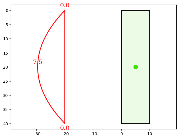
This produces a graphical representation of the shear stress \(\tau(z)\) distribution along the height of the rectangle.