
Second Order: Nonlinear Factors in Bar Attributes#
This example demonstrates how the local stiffness matrix and load vector of a bar element change when nonlinear geometric effects (Second-Order Theory) are considered. It serves as an extension of the previous example “Second Order: Matrix Approach”. For details on solving a complete Second-Order system using the matrix-based approach, please refer to that example.
The same cantilever system from the previous example is used here. It consists of a 4 m vertical cantilever column modeled with one bar, a point load at the free end, and a trapezoidal distributed load along its length.
Define the Structural System#
In this section, the static system is modeled. For a detailed step-by-step workflow, refer to the “Getting Started” example.
[1]:
from sstatics.core.preprocessing import (Bar, BarLineLoad, BarSecond,CrossSection,
                                         Material, Node, NodePointLoad, System)
from sstatics.core.calc_methods import SecondOrder
from sstatics.core.postprocessing.graphic_objects import ObjectRenderer, SystemGeo
import numpy as np

# 1. Define cross-section and material -> steel and HEA 240 profile
c_1 = CrossSection(0.00002769, 0.007684, 0.2, 0.2, 0.6275377)
m_1 = Material(210000000, 0.1, 81000000, 0.1)

# 2. Define nodes (cantilever system)
node_1 = Node(x=0, z=0, u='fixed', w='fixed', phi='fixed', rotation=np.pi/2)
node_2 = Node(x=0, z=-4, loads=NodePointLoad(x=0, z=182, phi=0, rotation=0))

# 3. Define bar
bar_1 = Bar(node_1, node_2, c_1, m_1, line_loads=BarLineLoad(
    pi=1, pj=1.5, direction='z', coord='bar', length='exact'))

# 4. Define system
system = System([bar_1])

# Show system graphic
ObjectRenderer(SystemGeo(system), 'mpl').show(show_axis=False)
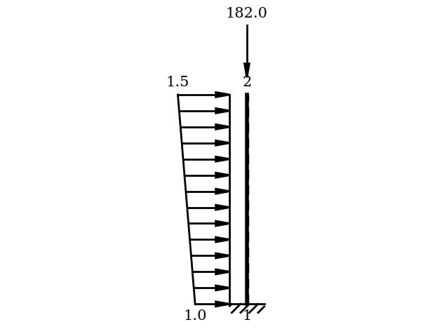
Compute the Longitudinal Force#
To include Second-Order effects, the average longitudinal force (f_axial) in each bar must be known. This value is obtained from the initial system solution and represents the mean axial force along the member.
For the current example (a single-bar system), only one axial force is returned. We select the first value from the list.
[2]:
# Compute average longitudinal force for the bar(s)
f_axial = SecondOrder(system).averaged_longitudinal_force[0]
Define the Second-Order Bar#
A bar considering Second-Order effects is defined similarly to a standard Bar, but with two key differences:
The approach (solver method) must be specified, e.g. ‘analytic’.
The average longitudinal force (f_axial) must be provided.
This allows the bar’s stiffness matrix and load vector to include geometric nonlinearity.
[3]:
bar_1_second = BarSecond(
    node_1, node_2, c_1, m_1, line_loads=BarLineLoad(
        pi=1, pj=1.5, direction='z', coord='bar', length='exact'),
    approach='analytic', f_axial=f_axial
)
Comparison of Linear and Nonlinear Behavior#
Now we can compare the stiffness matrices and load vectors between:
The First-Order (linear) bar
The Second-Order (analytic) bar
This illustrates how geometric nonlinearity modifies the element behavior.
[4]:
# Compare stiffness matrices
# for better visualization change print options
np.set_printoptions(
    precision=0,      # number of decimals
    suppress=True,    # suppress scientific notation for small numbers
)
print("Stiffness matrix (First Order):\n", bar_1.stiffness_matrix())
print('==================================================')
print("Stiffness matrix (Second Order - Analytic):\n", bar_1_second.stiffness_matrix())
Stiffness matrix (First Order):
 [[403410.      0.      0.     -0. 403410.      0.]
 [     0.   1090.  -2181.  -1090.     -0.  -2181.]
 [     0.  -2181.   5815.   2181.      0.   2907.]
 [    -0.  -1090.   2181.   1090.     -0.   2181.]
 [403410.     -0.      0.     -0. 403410.      0.]
 [     0.  -2181.   2907.   2181.      0.   5815.]]
==================================================
Stiffness matrix (Second Order - Analytic):
 [[403410.      0.      0.     -0. 403410.      0.]
 [     0.   1035.  -2161.  -1035.     -0.  -2161.]
 [     0.  -2161.   5714.   2161.      0.   2929.]
 [    -0.  -1035.   2161.   1035.     -0.   2161.]
 [403410.     -0.      0.     -0. 403410.      0.]
 [     0.  -2161.   2929.   2161.      0.   5714.]]
[5]:
# Compare load vectors
import numpy as np
np.set_printoptions(
    precision=3,      # number of decimals
    suppress=True,    # suppress scientific notation for small numbers
)
print("Load vector (First Order):\n", bar_1.f0())
print('=======================================')
print("Load vector (Second Order - Analytic):\n", bar_1_second.f0())
Load vector (First Order):
 [[ 0.   ]
 [-2.3  ]
 [ 1.6  ]
 [-2.7  ]
 [-0.   ]
 [-1.733]]
=======================================
Load vector (Second Order - Analytic):
 [[ 0.   ]
 [-2.3  ]
 [ 1.614]
 [-2.7  ]
 [-0.   ]
 [-1.748]]
Summary#
The stiffness matrix of the Second-Order bar includes additional terms dependent on the axial force (f_axial). This example highlights the influence of geometric nonlinearity on element-level quantities such as stiffness matrices and load vectors. It provides a detailed insight into how the BarSecond class modifies the bar attributes for Second-Order effects. For a full system-level Second-Order analysis, refer to the example: “Second Order: Matrix
Approach”.