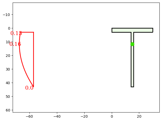
Stress: Stress in a T-Shaped Cross-Section

In this advanced example, we compute normal, bending, and shear stresses for a T-shaped cross-section, combining a flange and a web.

This demonstrates how to handle more complex geometries using the sstatics framework.

You can find the example as an executable Python file here.

Import Modules

We start by importing the required classes for defining the Stress object.

from sstatics.core.preprocessing import CrossSection
from sstatics.core.preprocessing.geometry.objects import Polygon
from sstatics.core.postprocessing import CrossSectionStress

Create Cross-Section

We define the T-shape as two polygons:

• Flange: horizontal top part

• Web: vertical connecting part

geometry = [
    Polygon([(0, 0), (30, 0), (30, 3), (0, 3), (0, 0)]),      # flange
    Polygon([(14, 3), (16, 3), (16, 43), (14, 43), (14, 3)])  # web
]

cs = CrossSection(geometry=geometry)

The CrossSection class calculates the geometric properties such as area, centroid, and boundaries.

Create Stress-Object

Using the previously defined cross-section, we create an instance of CrossSectionStress.

This object allows computation of normal stress (\(\sigma\)), bending stress (\(\sigma_b\)), and shear stress (\(\tau\)) for the section.

stress = CrossSectionStress(cs)

Define Applied Loads

We apply:

Axial force: \(N = 2\) Bending moment: \(M = 10\) Shear force: \(V = 10\)

N = 2   # axial force
M = 10  # bending moment
V = 10  # shear force

Geometric Parameters

The centroid \(z_s\) and the cross-section boundaries are used to determine stress distributions: Top distance to centroid: \(z_\text{top} - z_s\) Bottom distance to centroid: \(z_\text{bottom} - z_s\)

# Centroid location
z_s = cs.center_of_mass_z

# Cross-section boundaries
_, zb = cs.boundary()
z_top, z_bottom = zb[0], zb[1]

# Distances to centroid
dist_top = abs(z_top - z_s)
dist_bottom = abs(z_bottom - z_s)

print("=== T Cross-Section Example ===")
print("Centroid at z_s =", z_s)
print(f"Distance top to centroid: {dist_top}")
print(f"Distance bottom to centroid: {dist_bottom}")

=== T Cross-Section Example ===
Centroid at z_s = 11.617647058823529
Distance top to centroid: 11.617647058823529
Distance bottom to centroid: 31.38235294117647

Normal Stress

The normal stress due to axial force is uniform across the section:

# Normal stress: maximum occurs everywhere
print("Normal stress (maximum):", stress.normal_stress(N))

Normal stress (maximum): 0.011764705882352941

Bending Stress

The bending stress is calculated using:

\[\sigma_b(z) = \frac{M \cdot y}{I}\]

• Maximum bending stress occurs at the farthest distance from the centroid, either at the top or bottom fiber.

• If \(z\) is not specified, the method automatically returns the maximum bending stress.

# Automatically returns maximum bending stress
print("Bending stress (maximum):", stress.bending_stress(M))

# Explicitly at the largest distance from centroid (illustrative)
print("Bending stress at the largest distance from centroid:",
      stress.bending_stress(M, z=z_bottom))

Bending stress (maximum): 0.010353175572198118
Bending stress at the largest distance from centroid: 0.010353175572198118

Shear Stress

The shear stress distribution follows Jourawski’s formula:

\[\tau(z) = \frac{V \cdot S(z)}{I \cdot t(z)}\]

• Maximum shear occurs at the centroid.

• To visualize the shear distribution along the web, we discretize the section:

# Shear stress: maximum occurs at centroid
print("Shear stress (maximum at centroid):", stress.shear_stress(V))

Shear stress (maximum at centroid): 0.162453504934344

Now we want to plot the shear distribution along the web of the T-shaped section.

# Shear distribution for plotting along the web
stress.shear_stress_disc(v_z=V, z_i=3.01, z_j=43, n_disc=20)
stress.plot(kind="shear")