Second Order: Iterative Approach

This example demonstrates the iterative approach for performing a Second-Order analysis on a cantilever column. As in the previous example “Second Order: Matrix Approach”, the structure is a 4 m cantilever with a HEA 240 cross-section, subjected to a point load at the top and a trapezoidal distributed load along its length.

The iterative approach refines the equilibrium solution step by step until convergence is achieved. Instead of updating the element stiffness matrices directly, the equilibrium is reached by incrementally adjusting the nodal displacements and updating the system geometry in each iteration.

Concept of the Iterative Approach

In Second-Order theory, the system behavior depends on its deformed geometry. While analytic or matrix-based approaches include geometric effects directly in the stiffness matrix, the iterative method approximates these effects by repeatedly solving the system as the geometry changes.

Core idea:

1. Start with a First-Order analysis (undeformed geometry).

2. Compute displacements and internal forces.

3. Update node positions based on the results.

4. Re-solve the new system.

5. Repeat until the change in displacements between two iterations is smaller than a defined tolerance.

This iterative refinement gradually brings the structure into equilibrium in its deformed configuration, capturing geometric nonlinearities without directly modifying the stiffness matrices.

Program Workflow

The iterative process follows this workflow:

1. Create a SecondOrder instance with the structural system.

2. Call get_iteration_results() to start the iteration loop.

3. Define two key parameters:

   • Number of maximum iterations (e.g. 10)

   • Convergence tolerance (e.g. 0.001)

4. For each iteration:

   • Solve the current system.

   • Compare nodal displacements with the previous iteration.

   • update node coordinates

   • If the change < tolerance → stop.

   • Otherwise, update the system and continue.

5. Store intermediate systems and results for later inspection.

Define System

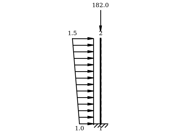
The same cantilever system from the previous example is used here. It consists of a 4 m vertical cantilever column modeled with one bar, a point load at the free end, and a trapezoidal distributed load along its length.

We first define the material, cross-section, nodes, bar, and assemble them into a System. For a detailed step-by-step workflow, refer to the “Getting Started” example.

# Import Modules
from sstatics.core.preprocessing import Bar, BarLineLoad, CrossSection, Material, Node, NodePointLoad, System
from sstatics.core.calc_methods import FirstOrder, SecondOrder
from sstatics.core.postprocessing.graphic_objects import ObjectRenderer, SystemGeo
import numpy as np

# Setting print options
np.set_printoptions(precision=3, suppress=True)

# Define cross-section and material
c_1 = CrossSection(0.00002769, 0.007684, 0.2, 0.2, 0.6275377)
m_1 = Material(210000000, 0.1, 81000000, 0.1)

# Define nodes
node_1 = Node(x=0, z=0, u='fixed', w='fixed', phi='fixed', rotation=np.pi/2)
node_2 = Node(x=0, z=-4, loads=NodePointLoad(x=0, z=182, phi=0, rotation=0))

# Define bar with trapezoidal line load
bar_1 = Bar(
    node_1,
    node_2,
    c_1,
    m_1,
    line_loads=BarLineLoad(pi=1, pj=1.5, direction='z', coord='bar', length='exact')
)

# Create system
system = System([bar_1])

# Visualize system
ObjectRenderer(SystemGeo(system), 'mpl').show(show_axis=False)

Running the Iterative Solver

We now start the iterative process with a maximum of 10 iterations and a convergence tolerance of 0.001. The process stops when either:

• 10 iterations are reached, or

• the maximum nodal displacement change between two steps is smaller than 0.001.

# Create SecondOrder object
sec_order_analysis = SecondOrder(system)

# Run iteratice process
sec_order_analysis.iterative_approach(iterations=10, tolerance=0.001, result_type='cumulative')
max_shift = sec_order_analysis.max_shift[-1]

Monitoring the Iteration Progress

The number of iterations actually performed can be checked via the attribute iteration_count. This allows you to confirm whether convergence was reached early or if the process reached the iteration limit.

print("Number of iterations performed:", sec_order_analysis.iteration_count)
print("Maximum displacement change in last iteration:", max_shift)
print("Convergence tolerance:", 0.001)

if max_shift < 0.001:
    print("Convergence criterion satisfied.")
else:
    print("Convergence not yet reached.")

Number of iterations performed: 3
Maximum displacement change in last iteration: 0.00020853608484659974
Convergence tolerance: 0.001
Convergence criterion satisfied.

Accessing Iteration Data

After solving the iterative process by calling get_iteration_results, several helper methods make it easy to explore the results:

Method	Description
iteration_count	Number of iterations performed
solver_iteration_cumulativ(i)	Returns total system response up to iteration i
results_iterative_growth(i, diff)	Returns only the incremental difference between iteration i–1 and i for a chosen result.
system_iterative(i)	Returns the system instance for iteration i
max_shift	Returns a list of the maximal shifts of the iteration process.

Bending Moment Evolution

We can now track how the bending moment at the fixed node (Node 1) evolves from the initial First-Order solution (iteration 0) to the final converged iteration.

Iteration 0 represents the initial undeformed solution that provides the starting point for the iterative process.

# Get solver objects
solver_initial = sec_order_analysis.solver_iteration_cumulative(0)
solver_final = sec_order_analysis.solver_iteration_cumulative(-1)

# Extract bending moment at Node 1
moment_initial = solver_initial.internal_forces[0][2][0]
moment_final = solver_final.internal_forces[0][2][0]


print("Initial bending moment at Node 1:", round(moment_initial, 3))
print("Final bending moment at Node 1 (after iteration):", round(moment_final, 3))
print("Change in bending moment:", round(moment_final - moment_initial, 3))

Initial bending moment at Node 1: 10.667
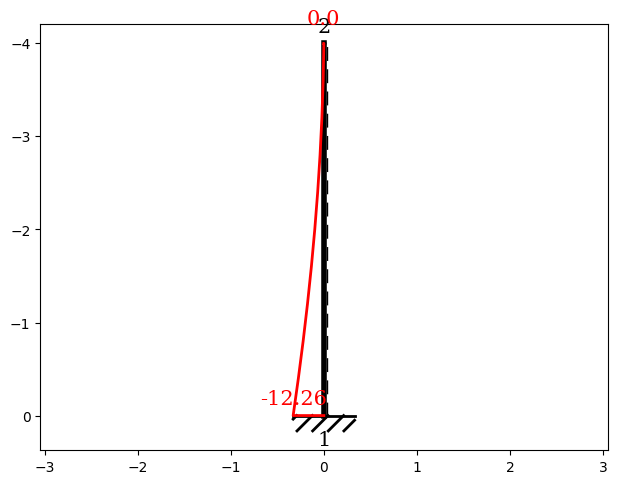
Final bending moment at Node 1 (after iteration): 12.261
Change in bending moment: 1.594

Plot of the last iteration step

The bending moment distribution can be visualized directly using the plot method from the SecondOrder class. To display the bending moment diagram, set the parameter kind='moment' and chose the correct approach (approach='iterative'). You can also select the iteration step you want to visualize. In this example we want to show the bending moment for the last iteration step (index=[-1])

sec_order_analysis.plot(approach='iterative', iteration_index=-1, kind='moment')

Incremental Changes in the Final Step

To analyze the final convergence step, we can return the iterative growth for this step. To be able to return the iterative growth, we have to run the start the iterative process for the result_type incremental. After the iterative process is finished, we can call the iterative growth between two iteration steps by using the function results_iterative_growth(). In this function it is possible to chose the the iteration step we want to analyse and the difference we want to see. In this example we want to see the iterative growth of the internal forces of the last iteration step.

# Run iteration process for the incremental result type
sec_order_analysis.iterative_approach(iterations=10, tolerance=1e-3, result_type='incremental')

# Get the iterative growth of the last iteration step for the internal forces
internal_forces_difference = sec_order_analysis.results_iterative_growth(-1, 'internal_forces')

# Incremental change in bending moment
moment_increment = internal_forces_difference[0][2][0]

print("Incremental bending moment change (last step):", round(moment_increment, 6))

Incremental bending moment change (last step): 0.227601