Force Method: Deformation of a simple frame

Demonstration of the Force Method for a simple frame

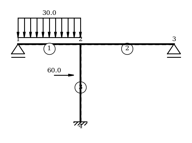
In this example, a small frame with three bars is analyzed using the Force Method. The method introduces redundant forces corresponding to the removed constraints (hinges) and computes the internal force distribution using influence coefficients (delta_i_j) and load coefficients (delta_i_0).

The system includes:

• Line and point loads on the bars

• Hinges introduced at specific bar ends

• Computation of redundant forces by solving A * x = b

You can find the example as an executable Python file here.

Define the Structural System

In this section, the static system is modeled. For a detailed step-by-step workflow, refer to the “Getting Started” example.

# 1. Import required modules
from sstatics.core.calc_methods import ForceMethod
from sstatics.core.preprocessing import (
    Node, Bar, Material, CrossSection, System, BarLineLoad, BarPointLoad
)
from sstatics.core.postprocessing.graphic_objects import ObjectRenderer, SystemGeo
import numpy as np

# 2. Define material and cross-sections
mat_1 = Material(3.0e7, 1, 1, 0.000012)
cs_1 = CrossSection(0.003125, 0.15, 0.5, 0.3, 1.0)
cs_2 = CrossSection(0.000675, 0.09, 0.3, 0.3, 1.0)

# 3. Define nodes
n1 = Node(0, 0, u="free", w="fixed", phi="free")
n2 = Node(2, 0)
n3 = Node(5, 0, u="free", w="fixed", phi="free")
n4 = Node(2, 2.5, u="fixed", w="fixed", phi="fixed", rotation=np.pi/2)

# 4. Define loads
line_load = BarLineLoad(pi=30, pj=30, direction="z")
point_load = BarPointLoad(x=60, position=0.6)
def_comp = 'moment'

# 5. Define bars
b1 = Bar(n1, n2, cs_1, mat_1, line_loads=line_load, deformations=def_comp)
b2 = Bar(n2, n3, cs_1, mat_1, deformations=def_comp)
b3 = Bar(n4, n2, cs_2, mat_1, point_loads=point_load, deformations=def_comp)

bars = [b1, b2, b3]

# 6. Create system
system = System(bars)

# Show system graphic
ObjectRenderer(SystemGeo(system, show_bar_text=True), 'mpl').show(show_axis=False)

Perform the Force Method

Next, we pass the modeled system to the ForceMethod class.

# 7. Initialize Force Method
force_method = ForceMethod(system)

Determine the Degree of Static Indeterminacy

Before creating a released system, it is necessary to determine the degree of static indeterminacy. This value can be obtained using the function degree_of_static_indeterminacy.

For our modeled system, the degree of static indeterminacy is:

print("Degree of static indeterminacy:",
      force_method.degree_of_static_indeterminacy)

Degree of static indeterminacy: 2

Create Released System

We now know that our modeled system is statically indeterminate of degree 2. The released system represents the corresponding statically determinate system of the original model.

To obtain such a system, certain restraints must be released. However, it is essential that the structure remains stable after doing so.

There are three available methods:

• modify_node() Modifies a support condition. The modeled node is passed to the function, and the specific degree of freedom to be released is defined.

• modify_bar() Modifies a bar by introducing a hinge. The modeled bar is passed to the function, and a hinge is added to release the corresponding internal restraint.

• delete_bar() Removes a bar from the structure. However, the software does not internally check the deformation contributions to verify whether removing a bar is structurally safe.

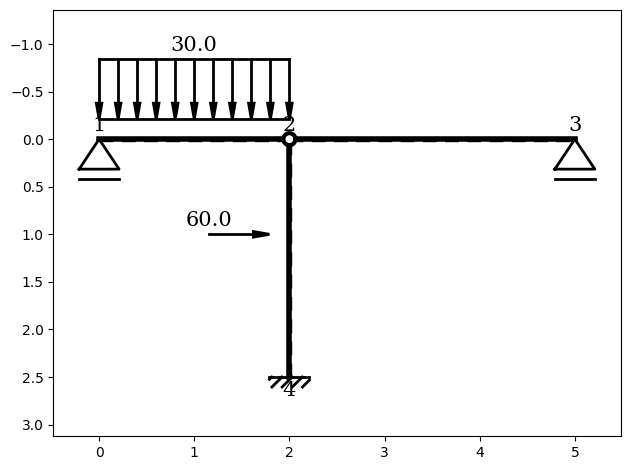
In this example, we choose to introduce a moment hinge at the end of bar 3 and bar 4.

# 8. Remove redundant degrees of freedom to form a statically determinate
# system
force_method.modify_bar(b1, hinge="hinge_phi_j")
force_method.modify_bar(b3, hinge="hinge_phi_j")

Check the Degree of Static Indeterminacy Again

Now we check the degree of static indeterminacy once more to verify that it is now equal to 0. A value of 0 indicates that the system is statically determinate, meaning the released system has been successfully created.

print("Degree of static indeterminacy:",
      force_method.degree_of_static_indeterminacy)

Degree of static indeterminacy: 0

The released system is now statically determinate.

Plot the Released System

It is possible to visualize the released system using plot_released_system(). This allows you to inspect the modified structure and verify which connections or supports were released.

# plot released system
force_method.plot_released_system()

Plot the Unit load States

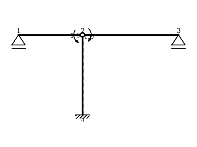
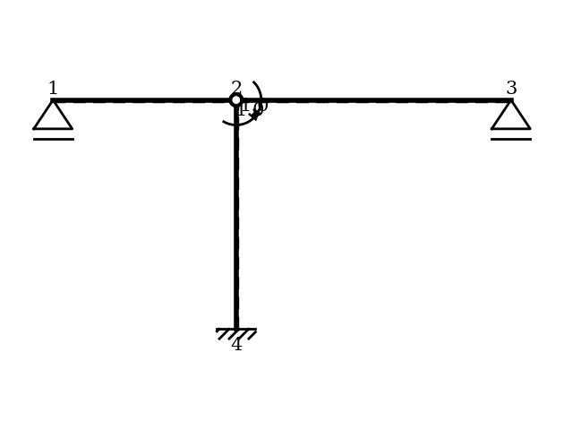
In this next step, we visualize the unit load states.

for system in force_method.uls_systems:
    ObjectRenderer(SystemGeo(system), 'mpl').show(show_axis=False)

Calculate the Influence and Load Coefficients

In the next step we compute the influence coefficients (German: Vorzahlen) and the load coefficients (German: Belastungszahlen). These values are needed to determine the unknown redundant reactions (X_i).

Use the functions influence_coef and load_coef to compute them.

• Load coefficients are collected in a vector (one entry per unit-load state). In this example two restraints were released, so there are two unit-load states and the load vector takes the form

  \(b = \left(\begin{array}{c} \delta_{10} \\ \delta_{20} \end{array}\right)\)

  where (\delta_{i0}) is the work (or deformation) produced in the main system by unit load state (i).

• Influence coefficients are stored in a square matrix because the unit-load states interact with each other. With two unit load states the influence matrix is

  \(A =\left[\begin{array}{cc} \delta_{11} & \delta_{12} \\ \delta_{21} & \delta_{22} \end{array}\right]\)

  where \(\delta_{ij}\) is the work (or mutual deformation) produced in unit load state (i) by unit load (j).

These quantities are assembled so that the unknown redundants \(\mathbf{X} = (X_1, X_2)^\top\) are found by solving the linear system \(\mathbf{A} \cdot \mathbf{X} = \mathbf{b}\)

# 9. Compute influence coefficients (delta_i_j = Vorzahlen)
#    and load coefficients (delta_i_0 = Belastungszahlen)
delta_i_j = np.array(force_method.influence_coef)
delta_i_0 = np.array(force_method.load_coef)

print(f"load coefficients (δ_i0):\n {delta_i_0}")
print(f"influence coefficients (δ_ij):\n {delta_i_j}")

load coefficients (δ_i0):
 [[ 0.00010667]
 [-0.00333333]]
influence coefficients (δ_ij):
 [[1.77777778e-05 1.06666667e-05]
 [1.06666667e-05 1.34123457e-04]]

Solve the System of Equations – Determine redundant forces

With the influence coefficients and load coefficients computed, the remaining step is to solve the linear system

\(A \cdot x = b\)

to obtain the redundant forces \(X_i\).

# 10. Display system of equations A * x = b
print("System of equations (delta_i_j * x = delta_i_0):")
for i in range(delta_i_j.shape[0]):
    row = " + ".join(f"{delta_i_j[i,j]:.4e}*x{j+1}"
                     for j in range(delta_i_j.shape[1]))
    print(f"{row} = {delta_i_0[i,0]:.4e}")

# Solve for redundant forces (x = unbekannte Kräfte)
x = np.array(force_method.redundants)
x1 = x[0][0]
x2 = x[1][0]

print("Redundant forces (x):")
for i in range(x.shape[0]):
    print(f"x{i+1} = {x[i, 0]:.6e}")

System of equations (delta_i_j * x = delta_i_0):
1.7778e-05*x1 + 1.0667e-05*x2 = 1.0667e-04
1.0667e-05*x1 + 1.3412e-04*x2 = -3.3333e-03
Redundant forces (x):
x1 = -2.195948e+01
x2 = 2.659913e+01

Validate Results

With the redundant forces determined, the internal force distribution of the statically indeterminate system can be reconstructed using the Force Method.

For demonstration, we compute the end bending moment of bar 1. The moment is obtained by superposition:

\(M = M_{0} + X_{1} \cdot M_{1} + X_{2} \cdot M_{2}\)

# 11. Validate results
from sstatics.core.calc_methods import FirstOrder

# Base system (released system)
solution_rls = force_method.solution_rls_system
forces_rls = solution_rls.internal_forces

# Unit load systems
solution_uls_1 = force_method.solution_uls_systems[0]
forces_uls_1 = solution_uls_1.internal_forces

solution_uls_2 = force_method.solution_uls_systems[1]
forces_uls_2 = solution_uls_2.internal_forces

# Retrieve bending moments at end of bar 1
# index [0] -> first bar in mesh
# index [5] -> moment at bar end
# index [0] -> scalar value
m0_j_b1 = forces_rls[0][5][0]
m1_j_b1 = forces_uls_1[0][5][0]
m2_j_b1 = forces_uls_2[0][5][0]

# Superposition to obtain final moment
m_j_b1 = m0_j_b1 + x1 * m1_j_b1 + x2 * m2_j_b1
print(f"Moment at end of bar 1 (Force Method): {m_j_b1}")

# Compare with the First-Order reference solution
solution_f0 = FirstOrder(system)
forces_f0 = solution_f0.internal_forces
m_j_b1_f0 = forces_f0[0][5][0]
print(f"Moment at end of bar 1 (FirstOrder): {m_j_b1_f0}")

# Verify agreement
print("Results match:", np.allclose(m_j_b1, m_j_b1_f0, atol=1e-2))

Moment at end of bar 1 (Force Method): -21.959480358995794
Moment at end of bar 1 (FirstOrder): 0.0
Results match: False

Visualize Moment Distribution

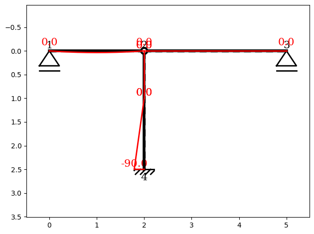
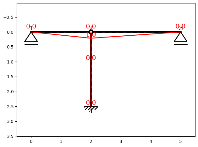
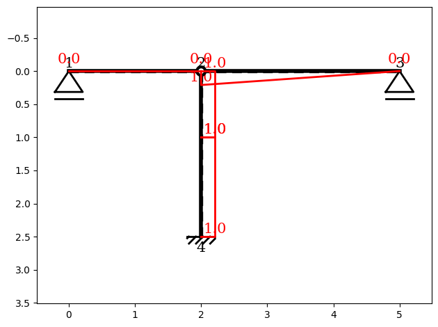
It is also possible to plot the internal force distributions of both the released system (RLS) and the unit load systems (ULS). The example below illustrates how to visualize the bending moment diagrams for these systems.

# 12. Optional visualizations
force_method.plot(system_mode='rls', kind='moment')    # released system
force_method.plot(system_mode='uls', uls_index=0, kind='moment')  # ULS 1
force_method.plot(system_mode='uls', uls_index=1, kind='moment')  # ULS 2

Inspecting the Work Matrix

To better understand how the values of δᵢⱼ (influence coefficients) and δᵢ₀ (load coefficients) are generated, we can inspect the internal work contributions of individual bars.

Example:

• uls_index_i = 0 → ULS 1

• uls_index_j = 1 → ULS 2

A detailed explanation of how the work_of methods operate can be found in “Principle of Virtual Forces: Relative Rotation”.

# 13. Inspection the work matrix
print("\nWork matrix for ULS1 × ULS2:")
print(force_method.work_matrix('bars', uls_index_i=0, uls_index_j=1))

print("\nWork contributions of bar b3 for ULS1 × ULS2:")
print(force_method.work_of(
    obj=b3,
    uls_index_i=0,
    uls_index_j=1,
    sum=False
))

Work matrix for ULS1 × ULS2:
[[0.00000000e+00 0.00000000e+00 0.00000000e+00 0.00000000e+00
  0.00000000e+00]
 [1.06666667e-05 0.00000000e+00 0.00000000e+00 0.00000000e+00
  0.00000000e+00]
 [1.23636480e-20 0.00000000e+00 0.00000000e+00 0.00000000e+00
  0.00000000e+00]
 [5.09262029e-21 0.00000000e+00 0.00000000e+00 0.00000000e+00
  0.00000000e+00]]

Work contributions of bar b3 for ULS1 × ULS2:
[[1.23636480e-20 0.00000000e+00 0.00000000e+00 0.00000000e+00
  0.00000000e+00]
 [5.09262029e-21 0.00000000e+00 0.00000000e+00 0.00000000e+00
  0.00000000e+00]]